How Names of Hybrid Orchids Work

Orchids are fascinating plants, and they are particularly known for allowing a lot of crossing between species. So much that there is a special system for naming hybrid orchids: greges.

A grex (plural “greges”) is a concept that applies only to orchids, and that replaces the concept of hybrid species, which is used otherwise in botany.

First a small detour about hybrid species, and how they are used. In nature, plants belong to species. So for instance, you may have at home some houseplant from the species Kalanchoe daigremontiana, which is also called “Mother of Thousands”.

Kalanchoe daigremontiana (by CrazyD)

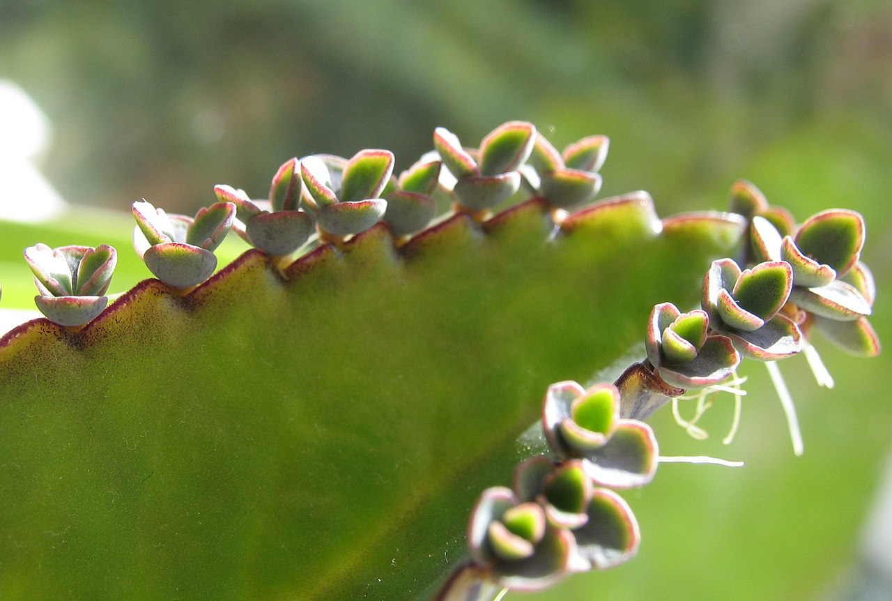
Now, this is a very beautiful plant which produces lots of little baby plants on the margin of the leaves, which tend to fall off and produces many more plants, explaining the common name. If you like this species, you may look for similar plants and come across Kalanchoe delagoensis, which has thinner leaves, but just as much little baby plants on them, and is therefore nicknamed “Mother of Millions”. In this case both “Kalanchoe daigremontiana” and “Kalanchoe delagoensis” are species and their names consist of the genus name (“Kalanchoe” for both) followed by a second word called the epithet. Together they form the species name.

If you’ve had kalanchoes than you know that they make beautiful little flowers, often in red. In fact, if you have both species, you may be able to cross-pollinate them to give a hybrid. This hybrid is called Kalanchoe houghtonii. This is not a species, but a hybrid species. Hybrid species are also called nothospecies. The important part is that species and nothospecies have the same naming conventions: A genus name followed by an Latin epithet, written in lowercase and usually in italics. We can write the situation down in a formula:

Kalanchoe houghtonii = Kalanchoe daigremontiana × Kalanchoe delagoensis

In this formula, the “×” is like a mathematical operation that takes two things (species or nothospecies) and returns a new thing (a nothospecies). This operation can be written in an abbreviated form as

Kalanchoe houghtonii = Kalanchoe daigremontiana × delagoensis

but that is purely a typographical detail that doesn’t change the meaning of the formula. In the following, I will avoid this type of shortcut.

When writing the name of a nothospecies, it is allowed to include a “×” sign before the epithet, as in “Kalanchoe ×houghtonii“, but that sign is optional, and in any case, for many species we are not certain that they are not hybrids of other species, so for most practical purposes, species and nothospecies can be considered the same thing. What should be noted is that the “×” sign is used in two different ways: As a binary operator that takes two (notho)species and returns a species, and as a prefix to denote that a name is a nothospecies. What may be even more confusing is that some people put a space between the “×” and the epithet, which gives “Kalanchoe × houghtonii”. To avoid confusion, we will never use “×” as a prefix – “×” will from here on always denote a binary operation.

Now, how is the situation for orchids? Well for botanists there is no difference, because botanists also use nothospecies to name hybrid orchids, and exactly the same rules apply. But botanists are only interested in hybrids that appear in nature. As for the thousands (or millions?) of hybrid orchids that are created in cultivation, there is a different naming system: the grex. An example is

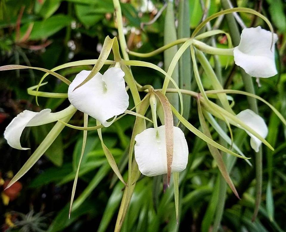
Brassavola Little Stars = Brassavola nodosa × Brassavola subulifolia

Brassavola Little Stars (by KrLo Javy)

The first thing to notice is that the epithet is not in Latin. In this case it is in English, but sometimes it’s in French like in “Paphiopedilum Ma Folie” or just the name of a person like in “Papilionanda Mimi Palmer”. Also, the epithet can consist of multiple words, and the words are capitalized. Also, italics are not used. But if those were the only differences, I would not have written this blog article. The real interesting part are the rules of naming, which I have summarized in this table:

Nothospecies
(any plant)
Greges
(only orchids)
IdempotenceA × A = AA × A = A
CommutativityA × B = B × AA × B = B × A
Associativity(A × B) × C = A × (B × C)–––––––

This requires some explanations. Let’s start with the rule “A × A = A”. In this notation each letter like A stands for a species, a nothospecies or grex. What this formula says is that if you cross a plant of type A with a plant of type A, you get another plant of type A. You cannot create a hybrid by starting with just one species. This is true for both nothospecies and greges, even if A is already a hybrid. Crossing a plant from nothospecies A with another plant from nothospecies A always gives a plant from nothospecies A. And the same is true for any grex A. The mathematical term for this rule of calculation is “idempotence”. Most mathematical operations we come across in daily life are not idempotent. “5 × 5 = 5” is not a true statement in mathematics, but

Kalanchoe daigremontiana × Kalanchoe daigremontiana = Kalanchoe daigremontiana

is a true statement in botany.

On to the second property. A × B = B × A. This means that it doesn’t matter whether A or B is the seed parent or the pollen parent. When two plants are crossed, one parent is the female parent (the “seed parent”) and one is the male parent (the “pollen parent”). In whatever way we cross A and B, we get the same result. Note that we have not even specified whether we write the seed parent or the pollen parent on the left or right of the sign “×”, but since our “×” always have the property of commutativity, it doesn’t matter. This rule works the same way for nothospecies as it does for greges. To give an example with greges this time, we can write

Brassavola nodosa × Brassavola subulifolia = Brassavola subulifolia × Brassavola nodosa

Both sides of this equation result in “Brassavola Little Stars”, and the equation is thus true.

For the third rule, we will now learn that nothospecies and greges work differently. Let’s look at nothospecies first. The rule

(A × B) × C = A × (B × C)

states that if we start with three types (A, B and C) and cross them, it does not matter which we cross first. We can cross A and B first (as written on the left side of the equal sign) or B and C first (as written on the right), the result is the same. In fact, we could even cross A and C first. How do I know that? By applying the rules of commutativity and associativity:

(A × B) × C = (B × A) × C = B × (A × C)

In this calculation, we first applied the rule of commutativity to “A × B” inside the parentheses, and then applied associativity to the result.

What is nice about the rule of associativity is that it allows us to omit the parentheses. “A × B × C” is a perfectly well-defined expression.

Imagine now that we have three species A, B and C. Which nothospecies can we construct from it? Let’s apply the operator “×” and define some new hybrid names:

D = A × B

E = B × C

F = A × C

G = A × B × C

Which other nothospecies can we define? A × A maybe? No, that’s the same as A. A × B × A maybe? No, that’s the same as A × B. You can convince yourself of that by first applying commutativity to get B × A × A, and then simplifying the expression using idempotence.

In fact, there are no more nothospecies we can define. Based on three species, we can only define four nothospecies.

As a little quiz: Given n species, how many nothospecies can we define? The answer is 2^n − n − 1. That’s because each nothospecies corresponds to one subset of the given set of species, which has n elements. There are 2^n subsets possible, but we must exclude the n given species (corresponding to sets with one element), and the set with zero elements (which doesn’t correspond to anything).

Mathematically, this all means that given a set of species S, the set S along with all nothospecies that can be derived from it forms the free semilattice generated by S. Don’t worry if “free semilattice” seems very complicated. It makes sense mathematically, but it would be too long to explain here.

Now let’s go over to the world or hybrid orchids and their grex names. Let’s start with three species A, B and C. As before we can define D = A × B, E = B× C and F = A × C. We can also define G = (A × B) × C, being careful to use parentheses, because “×” is not associative for greges. Which means that H = A × (B × C) is another grex.

Also, we can now define I = (A × B) × A. Since we don’t have associativity available, this does not simplify to A × B as was the case with nothospecies.

We can also define J = ((A × B) × A) × B, H = (((A × B) × A) × B) × A, and so on. And even something like ((((B × A) × A) × A) × A) × A cannot be simplified. What this means is that even starting with just two orchid species, we can in theory define an infinite number of new greges.

To give a an example of this, consider the following orchid greges:

B. Solstice Star = B. subulifolia × (B. nodosa × B. cucullata)

B. Little Yaki = (B. subulifolia × B. nodosa) × B. cucullata

I’ve abbreviated “Brassavola” as “B.” to make the formulas shorter.

What we can observe here is that Brassavola Solstice Star and Brassavola Little Yaki are both hybrids of the same three Brassavola species, but in a different order. And since they are greges and not nothospecies, they have different names.

Mathematically, a set of orchid species together with the (infinite) set of possible greges would form something like a “free non-associative semilattice”, but I don’t think mathematicians use the expression “non-associative semilattice”. I’m sure someone can help me find the correct mathematical term.

To conclude, I’d just like to point out that since so many orchids can be hybridized, there is never a shortage of grex names, and new hybrids get defined all the time. Orchid cultivators give all possible names to new hybrids, sometimes to honour someone, but sometimes just because a word is funny.

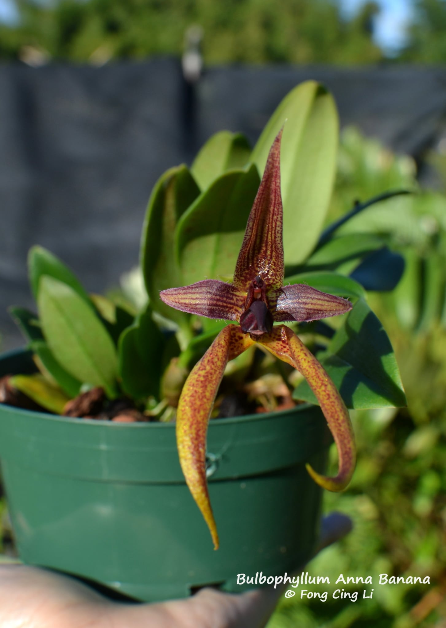
Just search for a funny word like “banana”, and you’ll find such gems as

Paphiopedilum Top Banana, Bulbophyllum Anna Banana, Calanthe Mana Banana, Lycaste Banana Pine, Oncidoglossum Banana Boat, Rhynchobrassoleya Banannarama, Vanda Habanananda, Zootrophion Pink Banana, Bulbophyllum Banana Split

and many many more.

Bulbophyllum Anna Banana (by Fong Cing Li Objio)

Game Dependency Graph: Day of the Tentacle

This is the game dependency graph for the game Day of the Tentacle (LucasArts, 1993).

A game dependency graph is a way to visualize certain computer games, which show all things that can be done in a game, connected in a way that shows their mutual dependencies. These graphs are also known as puzzle dependency charts, and they are most interesting for adventure games, as these games have the most interestingly interconnected puzzles.

For a more verbose overview of game dependency graphs see the blog entry about the graph for The Secret of Monkey Island. I’ve previously done the graphs for the first three Monkey Island games (1 2 3).

This time, I made a graph for the game Day of the Tentacle, another classic point-and-click adventure game from LucasArts, just like the Monkey Islands.

The special gimmick in this game is that you are playing three characters at the same time. While these characters are able to walk around through the same house, they do so with several hundred years separating them: Hoagie is in the 1790s, Bernard in the present (i.e., the 1990s), and Laverne in the 2190s, a time when evil tentacles rule the Earth. Your goal is to save the world. I’m not gonna say more about the plot here, but beware that the graph does contain tons of spoilers. You should have played the game before looking at it.

The three playable characters of the game are in different times, but you can still pass objects between them using the aptly named “Chron-O-Johns,” the time machines of the game that suspiciously look like portable toilets. This leads to some hilarious puzzles, such as the one where you have to leave a sweater in a washing machine in the present, only to get it back in the future, when it has shrunken to the size of a hamster. This is because you need the hamster-sized sweater for your hamster to wear, because otherwise your hamster feels too cold and wet to operate the big hamster-wheel-power-generator that you need to power your Chron-O-John to travel back in time. Anyway, the game is a lot of fun to play, and the chart below gives a good overview of all the clever puzzles that the makers came up with.

As always, write a comment below if you find an error; I will correct them all. And enjoy the graph!

I make these charts for fun and for the love of classic adventure games. If you like it, don’t hesitate to buy me a decaf. (I’m not gonna fall asleep, promised.) You can also write me at <kunegis@gmail.com> to get access to high resolution / vector versions of this chart, or to sponsor the creation of charts for other games.

You may also enjoy:

Game Dependency Graph: The Curse of Monkey Island

This is the game dependency graph for the adventure game The Curse of Monkey Island, also known as Monkey Island 3.

For an explanation of game dependency graphs, see the post about the game dependency graph for The Secret of Monkey Island (which is also known as Monkey Island 1).

I make these charts for fun.  If you like them, buy me a grog ‘n’ menthol.  You can also contact me on my Patreon to get access to high resolution / vector versions of this chart, or to sponsor the creation of charts for other games.

Chart as PDF

mi3


Edit History

2020-06-08 – EDIT Made Auger optional (as per Reddit comment) (v2)

2021-03-03 – EDIT updates to make it consistent with the upcoming chart for Day of the Tentacle (v3)

2021-03-17 – EDIT more updates due to the upcoming Day of the Tentacle chart (v4)

You May Also Like

Game Dependency Graph: Monkey Island 2: LeChuck’s Revenge

This post contains the game dependency graph for the game Monkey Island 2: LeChuck’s Revenge.

A little over a year ago, I created a graph representing the solution of the adventure game The Secret of Monkey Island.  This post does the same for the game’s sequel.

A game dependency graph is a way to represent the solution to an adventure game graphically:  Each action that can be performed in the game is a node in the graph, and two nodes are connected if one action must be performed before the other.  The leads to a directed acyclic graph – see the previous post for details.

I make these charts for fun.  If you like them, buy me a green drink. You can also contact me on my Patreon to get access to high resolution / vector versions of this chart, or to sponsor the creation of charts for other games.

Chart as PNG

mi2

EDIT 2020-06-01 Stylistic changes to make it consistent with the upcoming chart for MI3 (v3)

EDIT 2021-03-03 Changes in preparation with the upcoming chart for Day of the Tentacle. (v4)

EDIT 2021-03-17 More changes due to the upcoming Day of the Tentacle update (v5)

You May Also Like

Stu version 2.6 – Canonicalization

I just finalized version 2.6 of Stu, which adds the new feature of canonicalization.

Canonicalization allows several filenames to refer to the same file.  For a simple example, ‘config.h’ and ‘./config.h’ are now recognized as the same file.  (This was not the case in Stu 2.5 and earlier.)

The two rules of thumb for canonicalization are:

  • Canonicalization is mostly transparent for most uses, and works as expected.
  • Canonicalization never requires Stu perform system calls.  Therefore, handling of ‘..’ and symlinks is not performed.

The full rules are described in the manpage; the summary is:

(1) ‘.’ is recognized, as in the example given above.

(2) Multiple slashes are equivalent to a single slash, except when a filename starts with exactly two slashes.  (The extra case with names starting with exactly two slashes is in POSIX and is a remnant of “special” filenames on certain operating systems.)

In addition to this, there are three special rules:

(a) When a target to be canonicalized starts with ‘./’ followed immediately by a parameter, then this parameter will only match strings that do not start with a slash.  As an example, this makes it possible to have a rule with target ‘./config.h’ and another with target ‘$dir/config.h’, such that a dependency of ‘./config.h’ will match the first rule.

(b) A target of the form $a/xxx will match ‘/xxx’ with the parameter $a set to ‘/’.  This corresponds to the usual filename formation rules for files in the root directory.

(c) A target of the form $a/xxx will match ‘xxx’ with $a set to ‘.’.  Again, this is consistent with the way the ‘.’ filename works.

Extended Chart of Methods for Solving Rubik’s Cube

This is a network related to Rubik’s Cube.

rubik-chart.thumbnail-detail

It shows an overview of methods that can be used to solve the puzzle.  Each node in the network (dark rectangle) is an intermediate state, while each edge (annotated with rounded rectangles) is a step.

The chart can be read from top to bottom:  The topmost state represents the scrambled state of the cube; the bottommost state represent the solved puzzle.  Known methods to solve the cube, such as the CFOP or the Roux method, are shown as colored lines going from top to bottom.  Each connection (shown as gray lines) represents other theoretically possible methods to solve the puzzle.

Mathematically, each state is a subgroup of the overall Rubik’s Cube group, and each edge is a subgroup relationship.

More details and explanations about the chart are included in the chart itself, so I’m keeping this blog post short.

The full chart is available as a PDF file, and includes HTTP links for all references.  It has A0 format:

rubik-chart.thumbnail-allChart as PDF

As always, please report any error you may find.

I made this chart for fun, and because I love cubing and the math behind it.  If you like it, don’t hesitate to make a donation.

Network of Characters in Harry Potter

Here is another network.

This time, it’s the characters in the book series Harry Potter.

The nodes in this network are individual characters, and the edges are their relationships.  There are many different node types, to represent the different types of persons and animals, as well as various relationship types.  The complete list is given in the legend, and is pretty self-explanatory.

Since the universe of Harry Potter is gigantic, I have only included information included in the seven books.  Anything else, even if it is canon, is not shown.  I know that there’s much more information available about ancestors of those characters, as well as their children in some cases.  This is all not included.  Note that the graph is already quite large and complex, and some edges go all over the place.  Some persons are difficult to find too, because their placement may not be obvious.  Since many characters have relationships to many other characters, there is not perfect layout for all of this.  As a result, it is impossible to keep all groups of people together as one would like.  For instance, it would be nice to have all members of the Order of the Phoenix in one block, and each family in one block, and all Hogwarts teachers in one block, but those all overlap, and I had to make choices.  I hope the result is a good compromise.

Anyway, the network is also available as a PDF file, in which a text search can be performed.

To make the chart compact, I have omitted any titles like “Professor” and “Mr” in the names of people; you don’t have to notify me that the complete name of Nearly Headless Nick includes a “Sir” 🙂

I’m also aware that the overall layout is not perfect, but with a graph of this size, you have to make some tradeoffs, so I hope it’s still a very useful representation.

Another note:  I know that there are differences between the books and the movies; this network is about the books.

As always, I’m happy about corrections, so please write about any error you see.  (But keep in mind:  I’m not adding info that’s only available outside the seven books.)

The actual PDF file had exactly double the size of A0.  Apparently, there is no standardised name for this format (A−1?), but you could in principle print is as A0.  In the PDF, each text box is 1 cm high.

Finally:  This network contains spoilers for the Harry Potter series.  Also, if you’re not familiar with Harry Potter, then you’ll probably find this all boring . . . .

Chart as PDFChart as PNG

potter

I made this chart for fun and because I love Harry Potter.  If you like to help, please consider donating your thousand Galleon personal prize money an amount of your choice here.  Cheers!

EDIT 2020-02-15:  Small corrections (Version II)

EDIT 2021-03-20:  Add donation link in PDF (Version III)

Phylogenetic Tree of My Houseplants

Here’s a graph that is a little bit differentthan the usual: a tree. It shows all my houseplants, arranged by their taxonomic relationships.

A tree is a graph that does not contain cycles.  As such, trees lack some of the complex structure that characterizes other complex networks.  However, we can still make out some interesting “complex” properties, for instance the fact that a few families of plants have a large number of specimens in it (Cactaceae, Crassulaceae, Orchidaceae), while others have just a single member.

Each number in the graph (for instance [209]) refers to one plant.  In some cases, one number refers to multiple plants that are genetically identical, i.e., that I propagated from cuttings or similar.

All names shown are the taxonomically correct scientific names, for instance Euphorbia milii is what is sometimes called “crown of thorns” in English.

The names ending in “-aceae” are families (the grouping above the genus), and the names ending in “-ales” are orders (the grouping above the family).  Above orders, groupings use the usual scientific names “eudicots”, “monocots”, and “magnoliids”, which are mostly in English also in the scientific literature.

All my house plants are in the group “Angiosperms”, i.e., they are flowering plants.  I used to have a fern, but not anymore, and you can easily have conifers like Araucaria as a house plant, which are all outside of the Angiosperms.

I have resisted the temptation to add my house cat to the diagram, which of course would be a sister group to everything mentioned above.

All pictures are of my own plants, and made by myself.

flora.compressed

Game Dependency Graph: The Secret of Monkey Island

guybrush

This is something I already created a little more than a year ago, and only came around to publish now:  a game dependency graph.

The Secret of Monkey Island is a computer game from 1990 which I loved to play back in the day.  It is an adventure game, played with the mouse:  You play as a character named Guybrush Threepwood (shown on the right), and can walk around many different areas, interact with objects, people, and other things.  This is not an action game; you don’t need to perform actions at subsecond precision to win, but instead you must find out how to proceed in the story by performing the correct actions, such as using objects with other objects, talking to people, pushing things around, etc. Essentially, the whole game can be seen as a set of actions that must be performed.

The actions in this game cannot be performed in any random order, but are interrelated.  For instance, you need to pick up an object before you can use it.  Thus, we can model the whole game as a directed graph, which the actions being the nodes of the graph, and the dependencies as directed edges.  It is logically impossible for this dependency graph to have directed cycles, and thus this graph is a DAG, a directed acyclic graph.  In fact, this type of graph has already been considered, in particular under the name puzzle dependency chart; see that article by the creator of Monkey Island himself, Ron Gilbert.

This graph has many additional features in addition to just being a DAG – see below for an explanation.  The picture itself also includes a legend at the bottom.

SPOILER ALERT:  This post contains spoilers for pretty much all puzzles and for many easter eggs in The Secret of Monkey Island.

I make these charts for fun.  If you like them, buy me a grog.  You can also contact me at <kunegis@gmail.com> to get access to high resolution / vector versions of this chart, or to sponsor the creation of charts for other games.

Chart as PNG

mi1

Special Graph Features

The graph has some extra features that put it beyond “just a DAG”, which I’ll list in the following.

First of all, a note about the direction of edges:  The direction of edges is not indicated by little pointed arrows in the picture, but instead I follow the convention that all edges point down.  This is possible because the graph is acyclic.

Multiple Types of Actions

There are different types of actions that can be performed:  pick up, talk to, push, etc.  Each of these is represented by a differently colored node.

  • Rarely used commands are all shown in blue – remember that this is the first Monkey Island game, which had much more commands than later ones.  Commands like “push” and “pull” are used only a few times in the game (but sometimes in a clever way, for instance to “rotate” the safe handle and the balanced stones.)
  • Commands like “open” and “go to” are only shown if they have a game-relevant consequence.  I don’t include all doors you have to open just to go through the game.
  • I also don’t include all the people you can talk to.  Almost all of these dialogues are optional, and would just be isolated nodes in the graph.  I only make an exception for really, really important dialogues, such as with the Voodoo Lady.
  • There is a single way to die in game, which is represented as a black node, and obviously cannot have any outgoing edges.  It is located in the underwater scene in Part I.  (Note that Monkey Island avoids death as a general rule – the inclusion of this is more of an easter egg, rather than actual gameplay, in particular because it will only happen if the player cannot exit the underwater scene in ten minutes, which isn’t too difficult to do.)
  • There is also a way to get stuck in the game, by spending all pieces of eight on the broken grog machine.  This too is indicated by a black node.

Multiple Solutions

Some puzzles in this game have multiple solutions.  This is reflected in the graph by dashed lines that converge on a little circle.  This happens only a few times:

  • In order to enter the forest in Part I, one of two things must be done:  (1) buy the map, or (2) follow the storekeeper to the forest.  Once the forest can be entered, both the treasure and the Sword Master can be found without further help, but one of those two actions must be performed, because otherwise Guybrush refuses to enter the forest.
  • The option to ask the storekeeper to to the Sword Master (see previous point) can be unlocked in two ways:  (1) By talking to the important-looking pirates, or (2) by buying the sword from the storekeeper.
  • One of four different objects made out of cloth or paper can be used in the recipe puzzle in Part II:  the business card, the map (which is optional), or one of the two T-shirts.  The player can also put all of them into the pot in order to make the inventory shorter, since you don’t need them again.
  • The dam in Part III can be burst in four different ways:  (1) using the lens with the sun, (2) using the spyglass with the rock, (3) using the cannonball with the rock, and (4) using the magnetic compass with the rock.  This also means that getting the spyglass from the fort is completely optional, even though it can be used in two different ways to burst the dam.

“Action-Like” Puzzles

Some “action-like” puzzles in the game do not fit into the “dependency graph” approach, and are represented as a single node, even though the player must perform a little bit more than a single action.  These cases are shown in red in the graph.  These include: learning and applying swordfighting insults, navigating through the forest maze, following the store keeper to the swordmaster (which is optional), haggling with Stan, and tricking the storekeeper in order to steal the note of credit.

(Since the graph doesn’t say how to solve these puzzles, they are the only part of the game not spoilered by this post.)

Some puzzles are timed, i.e., you have do perform an action with correct timing, for instance tickling the ghost pirate’s feet with the ghost feather.  These are shown in orange.

Areas

The game is divided into what I call areas, and which are separated by dashed lines in the graph.  What I call an “area” is a set of rooms between which the player can navigate freely, and thus the player will always be in a single at a particular time, and will need to perform specific actions to enter another area.  In the beginning of the game, areas correspond to individual parts of the game, e.g., when the player can finally leave Mélêe Island™, after which Part II starts, and the player is now on the ship.  Each area can be seen as its own game with its own dependency graph.  There are also what I call “subareas” in the game, which happens when you enter an area (usally a single room), which, when exited, leads you back to the previous areas – these subareas are shown as dashed rectangles.  There are two of them: the seafloor scene in Part I, and being captured by the cannibals in Part III.  The ending of the game can be seen to consist of three consecutive small areas.

Network Analysis

We can now finally perform some network analysis.  Of course, a proper network analysis would be more interesting if we had multiple games to analyse, so I’ll restrict myself to things that can be gleaned “by hand”, e.g., without using a computer analysis.

Things You Can Do Immediately

Nodes that don’t have any incoming edges (i.e., no edge coming into them from above) are things you can do immediately when you enter an area.  You can think of there being implicit edges from the action that starts the area to all such nodes, but we don’t draw them because they don’t add any information, and would just clutter the graph.

Optional actions

Nodes in the graph that are not connected downward to the end of the game are optional, i.e., you don’t need to do them to win the game.

This includes talking to the important-looking pirates, talking to the sheriff in the alley, using a breath mint, putting money in the grog machine, getting the PTA minutes from the three pirates, playing with the rat, talking to the Voodoo lady, following the storekeeper to the swordmaster, opening the chest in the bedroom on the ship, picking up and reading all memos on Monkey Island, walking to the edge on the top of Monkey Island and falling down, and destroying the ship.

Of course, many of these are integral to the game’s storytelling, so you should do them – after all, exploring everything is what these kinds of games are all about.  (For destroying the ship, you get two slightly different endings depending on whether you did it or not.)

Redundant Transitive Edges

The graph is not a transitive reduction:  Certain dependency edges could be removed without changing the situation.

For instance in Part I, you need the pieces of eight to buy the sword, and you need the sword to train with Captain Smirk.  Thus, we can infer that you must have the pieces of eight when you train with Captain Smirk, and could thus omit the link from the pieces of eight to Captain Smirk.

In this case, we include such links because of the storytelling:  You need to give pieces of eight to Captain Smirk, and thus they are a logical dependency, even though it is impossible to not have the pieces of eight if you already have the sword.

Linear vs Parallel Gameplay

You can see in the graph that the game has distinctly different phases, purely based on the structure of the dependency graph:

The beginning is very dense with many possible parallel paths – as you start to explore the first area (Mêlée Island), you can do many things in parallel.

The end of the game, on the other hand, is much more linear:  The thirteen last actions (starting at “use jug o’grog with dish” in the pirate ship) must all be performed in the given order.

Diversity of Puzzles

Clearly, the puzzles in the beginning of the game are much more varied than those at the end.  The last “action-like” or “rarely used command” puzzle is the navigation through the underground maze in Part III – after that it’s just walking, talking, picking up objects, and using objects until the end of the game. The last action in the game however, is at least timed, so there’s that.

Compare that to the start of the game, which includes all possible commands in some way, all along with going through a maze, following a non-player character, almost dying underwater, and the whole insult swordfighting section.

(This is subjective of course, and I’d like to see how other games compare.)

Size of the Game

We can also use the graph to measure the “size” of the game.  There are 153 154 nodes in the graph (if I counted correctly), but since I haven’t done this for any other game, I can’t compare that number.

(Of course, this does not take into account the “action-like” sequences, which are much more present in this game than in other games of the genre.)

End Notes

If you haven’t played this game:  It is supported by ScummVM.  (There is also a remake which I haven’t tried, but you’d better be playing the original version, with those lovely pixely graphics.)

I also want to do this type of analysis for other games.  Candidates are:  Monkey Island 2 and 3, Day of the Tentacle, Flight of the Amazon Queen, The Dig, Full Throttle, Sam and Max, Simon the Sorcerer, and maybe something like Broken Sword.  Oh, and I would love to do Thimbleweed Park too (haven’t played it yet!).  (If I have time of course – this is not the type of analysis that they give you gigantic grants for, as fun as it is.)

If there are things that should be corrected in the graph, please drop a comment.

Fun fact:  the original Amiga version of the game came on four diskettes, and is only 18.5 times larger than the full-size image above. (If my calculations are correct)

You May Also Be Interested In

Edit Log

EDIT 2019-01-18:  Added one more optional action that I missed

EDIT 2019-01-18:  Added the death node in the underwater scene

EDIT 2019-01-18:  Added PDF version

EDIT 2019-01-19:  Added a link to Ron Gilbert’s page on puzzle dependency charts

EDIT 2019-01-21:  Divided a dashed box into “mansion”/”underwater” scenes; small adjustments in the chart (v3)

EDIT 2019-01-21:  Added note that not all dialogues are included in the graph

EDIT 2019-01-21:  Added getting stuck by spending all money on the grog machine; added “enter forest” as a node which can be achieved by either following the store keeper, or by buying the map; made clear that the poisoned meat can also be produced via the pot o’ stew; rearranged nodes

EDIT 2019-01-22:  Made the legend better (v6)

EDIT 2019-01-23:  Added bullet point about the two ways to enter the forest in Part I

EDIT 2019-02-03:  For following the storekeeper to the Sword Master:  the puzzle has multiple solutions (Thanks LogicDeLuxe from the Thimbleweed Park forums)

EDIT 2019-03-11:  Fix a typo

EDIT 2020-04-15: Stylistic changes to make it consistent with the upcoming MI2 graph (v13)

EDIT 2020-06-01:  Stylistic changes to make it consistent with the upcoming MI3 graph, other small changes  (v14)

EDIT 2021-03-03:  Many changes made in proparation for creation the map for Day of the Tentacle.  This includes new colors for push/pull, open/close, labels inside each area to show the location where it takea place, more edge colors to denote changed endings, hints, and optional actions.  (v15)

EDIT 2021-03-17:  More changes to be in line with Day of the Tentacle. (v16)

EDIT 2021-09-28:  Small tweaks and corrections based on feedback. (v17)

The Long Story of a Single Research Dataset

Let’s take a look at how a single dataset has spread from researcher to researcher over the years. It’s this network:

celegans-analysis

Analysis of the C. elegans metabolic network, from (Jeong et al. 2000)

In the KONECT project, we collect datasets that are in the form of networks, i.e., consist of interconnections between all kinds of things.  Recently, we added a network from biology: the metabolic network of Caenorhabditis elegans.  It represents information about the biochemistry of a certain roundworm, Caenorhabditis elegans, which was first discovered in soil in Algeria in 1900, and has since become one of the most-studied lifeforms (see here for why).

While preparing this dataset, I researched the history of the dataset itself, as I always do in order to have correctly labeled data. It turned out that this dataset has spread through the academic world, crossing the boundaries of multiple disciplines, and appearing in multiple formats in various studies.  Here’s my summary of the dataset’s history, as far as I can reconstruct it:

Genome Sequencing

Our story starts at the end of the 1990s. Cenorhabditis elegans is a model organism, i.e., a species used extensively for research.  In fact, it was the first multi-cellular organism to have its genome sequenced.  The project to sequence the full genome of C. elegans took decades, and was finalized in 1999, as summarized in this paper:

[1] R. K. Wilson. How the worm was won. The C. elegans genome sequencing project. Trends Genet., 15(2):51–8, 1999.

The resulting genome is about 97 megabytes large, and includes more than 19,000 proteins.

What Is There: Metabolic Reconstruction

Only one year later, in 2000, the genome of C. elegans is included in a project called What Is There, or just WIT.  Information about this project can be found in this paper:

[2] Ross Overbeek, Niels Larsen, Gordon D. Pusch, Mark D’Souza, Evgeni Selkov Jr., Nikos  Kyrpides, Michael Fonstein, Natalia Maltsev, and Evgeni Selkov. WIT: Integrated system for high-throughput genome sequence analysis and metabolic reconstruction. Nucleic Acids Res., 28(1):123–125, 2000.

Unfortunately, the URLs of this project are not accessible anymore:

However, we can glean information about the project from the article:

“The WIT (What Is There) system has been designed to support comparative analysis of sequenced genomes and to generate metabolic reconstructions based on chromosomal sequences and metabolic modules from the EMP/MPW family of databases. This system contains data derived from about 40 completed or nearly completed genomes.”

Network Science

Also in the year 2000, Hawoong Jeong and colleagues from Notre Dame (Indiana, USA) used the datasets from the WIT project in the following article:

[3] Hawoong Jeong, Bálint Tombor, Réka Albert, Zoltan N. Oltvai, and Albert-László Barabási. The large-scale organization of metabolic networks. Nature, 407:651–654, 2000.

To cite the paper:

“[…] We present a systematic comparative mathematical analysis of the metabolic networks of 43 organisms representing all three domains of life. We show that, despite significant variation in their individual constituents and pathways, these metabolic networks have the same topological scaling properties and show striking similarities to the inherent organization of complex non-biological systems.”

One of the 43 organisms is, of course, C. elegans.

Being an article in the then-emerging field of Network Science, this is the first version of our dataset that is actually a network.  To be precise, it is a metabolic network.

Community Detection

In 2005, Jordi Duch and Alex Arenas take the datasets from the 2000 paper in order to study community detection:

[4] Jordi Duch and Alex Arenas. Community detection in complex networks using extremal optimization (arXiv version). Phys. Rev. E, 72(2):027104, 2005.

In this article, seven network datasets from different sources are used, including the metabolic network of C. elegans.  (Another of the seven datasets is the famous Zachary karate club network dataset.)

To cite the article:

“We have also analyzed the community structure of several real networks: the jazz musicians network [27], an university e-mail network [11], the C. elegans metabolic network [28], a network of users of the PGP algorithm for secure information transactions [29], and finally the relations between authors that shared a paper in cond-mat [30].”

We can only guess why these particular datasets were chosen, but the fact that they are from different domains must have played a role, and the fact that in 2005, not many network datasets were easily available, as is the case nowadays.

The dataset as used in the paper is made available on the website of Alex Arenas.

Discrete Mathematics and Theoretical Computer Science

In 2011, the 10th implementation challenge of the Center for Discrete Mathematics and Theoretical Computer Science (DIMACS 10) starts. In this challenge, participants must implement graph partitioning and graph clustering algorithms. After the end of the challenge, participants present their results at a DIMACS conference in 2012.  A book including all algorithm descriptions and other papers is published in 2013:

[5] David A. Bader, Henning Meyerhenke, Peter Sanders, Dorothea Wagner (eds.). Graph Partitioning and Graph Clustering. 10th DIMACS Implementation Challenge Workshop. February 13-14, 2012. Georgia Institute of Technology, Atlanta, GA. Contemporary Mathematics 588. American Mathematical Society and Center for Discrete Mathematics and Theoretical Computer Science, 2013.

In the contest, many real-world network datasets are made available for participants to use. Among them is the C. elegans metabolic network, as taken from Alex Arenas’ website.  To quote the contest website:

“The following four datasets are taken from http://deim.urv.cat/~aarenas/data/welcome.htm, with kind permission of Alex Arenas, Dept. Enginyeria Informatica i Matematiques (Computer Science & Mathematics), Universidad Rovira i Virgili.”

The full dataset is available for download from the DIMACS10 website, in the data format used by the contest.

The KONECT Project

In 2018, the dataset is incorporated in the KONECT project, where it is, as of this writing, one out of 1326 such network datasets.

[6] Jérôme Kunegis. KONECT – The Koblenz Network Collection (CiteSeerX version). In Proc. Int. Conf. on World Wide Web Companion, pages 1343–1350, 2013.

In KONECT, we have extracted the C. elegans metabolic network dataset from the DIMACS10 website.  It is now also available for download from its KONECT page, in the KONECT format, which is used for all 1326 KONECT datasets. Additionally, the KONECT page of the dataset shows the values of 33 network statistics, and 45 plots.

Conclusion

This particular dataset has thus undergone the steps

Genome
↓
What Is There
↓
Notre Dame
↓
Duch & Arenas
↓
DIMACS10
↓
KONECT

The dataset has gone through all these steps, being downloaded and adapted for each particular project. Even though the researchers at each step (including myself) could have taken the dataset from previous steps, they didn’t. The reason may simply be simplicity in downloading the data, and a lack of knowledge about the full prevenance of the data.

Some readers may have noted that the dataset is also included in KONECT in a form directly extract from Alex Arenas’ website. This has been in KONECT for several years, but in fact, the two networks are not identical:  They have a different number of edges, although the number of nodes is the same. That difference is also the reason why we keep both version in KONECT. We don’t know what exactly the DIMACS10 project has done with the data. We know that multiple edges as available in the version of Alex Arenas have collapsed, but that still does not explain the difference. In light of such slight differences, we can only recommend to researchers analysing networks to properly cite the source of their dataset, and correctly document which transformations have been applied to the datasets. Even though this dataset is not one of the most famous (that award probably goes to the Zachary karate club), I would guess that the length of the chain of reuse is comparable for both.

Disclaimer

This chain of dataset sharing does of course not represent the full list of ways in which the dataset was made available, let alone used. In fact, the cited papers are not necessarily the first papers to perform a specific type of analysis – this chain of paper only represents how the dataset was shared, from the original dataset to KONECT. Note that the dataset was also shared in other ways that did not end up in KONECT. For instance, the dataset was used by Petter Holme and colleagues (in collaboration with Hawoong Jeong) for their 2003 article on detecting subnetworks, which used the version from the WIT project. Also, the dataset is available at the ICON project, and was extracted directly from Alex Arenas’ website there.  (Note: we can’t seem to get a direct link to that particular dataset in ICON – it can be found easily by searching for it.)

This text is likely to contain errors and omissions – please comment below, and I will correct them.  I remember that Albert-László Barabási had a separate page which may have contained the data too, but I can’t find it right now.  Maybe it was at https://www3.nd.edu/~networks, which is not reachable now?

EDIT 2018-04-18:  Added information via Petter Holme to the disclaimer, mentioning his 2003 paper.

EDIT 2018-04-20:  Fixed typos; change a formulation to make clear article [1] is a summary of the work, not the work itself; use quotation marks consistently.

EDIT 2018-05-08: Fixed typos; replaced “different” by “the same” in the description of the other dataset which is also in KONECT (Thanks Thomas)

EDIT 2018-06-11: Fixed year number in first sentence of section “Community Detection” (“2005 paper” → “2000 paper”)