My Shell Coding Conventions

When writing shell scripts, it is worth it to pay attention to details.

Here are the conventions I use when writing shell scripts.  These rules are taken from the coding conventions in Stu project, and are further maintained there.  I have omitted points that are specific to Stu.

Here’s the list:

• Only use POSIX features of the shell and of standard tools. Read the manpage of a tool on the POSIX website,  rather than your locally installed manpage, which is likely to describe extensions to the tool without documenting them as such.
• Sed has only basic regular expressions. In particular, no |, +, and no escape sequences like \s/\S/\b/\w. The -r and -E options are not POSIX; they are GNU and/or BSD extensions. A space can be written as [[:space:]]. + can be emulated with \{1,\}. There is no way to write alternatives, i.e., the | operator in extended regular regular expressions. (Note: there are rumors that -E is going to be in a future POSIX standard; I’ll switch to -E once it’s standardized.) Also, the b and t commands must not be followed by a semicolon; always use a newline after them when there are more commands.
• Grep does have the -E option for extended regular expressions. Grep is always invoked with the -E or the -F option. (Using basic regular expressions with Grep is also portable, but I don’t do it.)
• date +%s is not mandated by POSIX, even though it works on all operating systems I tried it on. It outputs the correct Unix time. There is a hackish but portable workaround using the random number generator of awk(1).
• Shell scripts don’t have a filename suffix. Use #! /bin/sh and set the executable bit. The space after ! is not necessary, but is traditional and I think it looks good, so I always use it.
• test does not support the -a option. Use && in the shell instead. POSIX has deprecated test -a.
• The “recursive” option to programs such as ls(1) and cp(1) is -R and not -r. -r for recursive behavior is available and prescribed by POSIX for some commands such as rm(1), but it’s easier to always use -R. Mnemonic: Output will be big, hence a big letter. The idiomatic rm -rf is thus not recommended, and rm -Rf is used instead.
• I use set -e. I don’t rely on it for “normal” code paths, but as an additional fail- safe. It does not work with $() commands that are used within other commands, and it also does not work with pipelines, except for the last command. When you use $(), assign its result to a variable, and then use its result from that variable. Using $() directly embedded in other commands will make the shell ignore failure of the inner shell. There is no good solution to the “first part of pipeline fails silently” problem.
• Use $(...) instead of `...`. It avoids many quoting pitfalls. In shell syntax, backticks are a form of quote which also executes its content. Thus, characters such as other backticks and backslashes inside it must be quoted by a backslash, leading to ugly code. $(...) does not have this problem. Also, in Unicode ` is a standalone grave accent character, and thus a letter-like character. This is also the reason why ` doesn’t need to be quoted in Stu, like any other letter. The same goes for ^ and the non-ASCII ´.
• Double-quote all variables, except if they should expand to multiple words in a command line, or when assigning to a variable. Also, use -- when passing variables as non-option arguments to programs. E.g., write cp -- "$filename_from" "$filename_to". All other invocation styles are unsafe under some values of the variables. Some programs such as printf don’t have options and thus don’t support or need --.
• Always use IFS= read -r instead of read. It’s the safe way to read anything that’s \n-delimited.
• To omit the trailing newline with echo, both -n and \c are non-portable. Instead, use printf. In general, printf is an underused command. It can often be used judiciously instead of echo. Note that the format string of printf should not start with a dash. In such cases, use %s and a subsequent string, which can start with a dash.

 

Google Is the Largest ‘Web Tracker’, but by Far Not the Only One

We performed a study about web tracking.

Web tracking refers to the very widespread practice of websites embedding so-called web trackers on their pages.  These have various purposes, such as optimizing the loading of images, or embedding additional services on a site.  The best known examples are the “Facebook buttons” and “Twitter buttons” found on many sites, but the most widespread ones are by far those from Google, which in fact operates a multitude of such “tracking services”.  There are however many more – what they all have in common is that they allow the company that runs them to track precisely which sites have been visited by each user.

Web trackers have been well-know for quite a time, but until now no web-scale study had been performed to measure their extent.  Thus, we performed a study about them. We analysed 200 terabytes of data on 3.5 billion web pages.

The key insights are:

• 90% of all websites contain trackers.
• Google tracks 24.8% of all domains on the internet, globally.
• When taking into account that not all web sites get visited equally often, Google’s reach is even higher:  We estimated that 50.7% of all visited pages on the web include trackers by Google.  (Ironically, we estimated this by using PageRank, a measure initially associated with Google itself.)
• The top three tracking systems deployed on the web are all operated by Google, and use the domains google-analytics.com, google.com, and googleapis.com.
• The top three companies that have trackers on the web are Google, Facebook, and Twitter, in that order.
• These big companies are by far not the only companies that track:  There is a long tail of trackers on the web – 50% of the tracking services are embedded on less than ten thousand domains, while tracking services in the top 1% of the distribution are integrated into more than a million domains.
• Google, Twitter and Facebook are the dominant tracking companies in almost all countries in the world.  Exceptions are Russia and China, in which local companies take the top rank. These are Yandex and CNZZ, respectively. Even in Iran, Google is the most deployed tracker.
• Websites about topics that are particularly privacy-sensitive are less likely to contain trackers than other websites, but still, the majority of such sites do contain trackers.  For instance, 60% of all forums and other sites about mental health, addiction, sexuality, and gender identity contain trackers, compared to 90% overall.
• Many sites contain more than one tracker.  In fact, multiple trackers are so common that we were able to determine clusters of trackers that are often used together by individual sites – these allow us to automatically detect different types of trackers such as advertising trackers, counters and sharing widgets.  (See the picture above.)

Not all trackers have the explicit purpose of tracking people: Many types of systems perform useful services in which tracking is a side effect.  Examples are caching images, optimizing load times, enhancing the usability of a site, etc. For many of these systems, webmasters may not be aware that they allow tracking.

Note:  The study was performed using data from 2012 by the Common Crawl project.  Due to the fact that their crawling strategy has changed since then, newer data in fact represents a smaller fraction of the whole web.

The study was performed by my colleague Sebastian Schelter from the Database Systems and Information Management Group of the Technical University of Berlin, and myself.

The article is published in the Journal of Web Science, and is available as open access:

1. Sebastian Schelter and Jérôme Kunegis (2018), “On the Ubiquity of Web Tracking: Insights from a Billion-Page Web Crawl”, The Journal of Web Science: Vol. 4: No. 4, pp 53–66.

The full dataset is available online on Sebastian’s website, and also via the KONECT project.

 

The Build System Stu in Practice

I haven’t blogged in a while about the Stu build system.  Stu is a piece of software written by myself at the University of Namur that we use to run the calculations of network statistics in the KONECT project, build Latex documents, and do all other sorts of data manipulation, and more.  The Stu build system is a domain-specific programming language used to build things.  This is similar to the well-know Make system, but can do much more.  In the KONECT project, we use it in ways that are impossible with Make.  In this post, I will show a very short snippet of a Stu script, as it is used in KONECT, and will explain what it does line by line.

Here is the snippet:

#
# Diadens
#

@diadens: @diadens.[dat/NETWORKS_TIME];

@diadens.$network:  plot/diadens.a.$network.eps;

plot/diadens.a.$network.eps: 
        m/diadens.m 
        $[ -t MATLABPATH]
        dat/stepsi.$network 
        dat/statistic_time.full.(diameter avgdegree).$network
{
        ./matlab m/diadens.m 
}

This code is written in Stu, and is used as shown here in KONECT.  It is part of the (much larger) file main.stu in the KONECT-Analysis project. I have left in the comments as they appear in the original.  In fact, comments in Stu start with #, and you can probably recognize that the first three lines are a comment:

#
# Diadens
#

The name “Diadens” refers to diameter-density; we’ll explain later what that means.

The comment syntax in Stu is the same as in many other scripting languages such as the Shell, Perl, Python, etc.  Until now, there’s nothing special.  Let’s continue:

@diadens: @diadens.[dat/NETWORKS_TIME];

Now we’re talking.  In order to explain this line, I must first explain the overall structure of a Stu script:  A Stu script consists of individual rules.  This one line represents a rule in itself.  Of course, rules may be much longer (as we will see later), but this rule is just a single line. As a general rule, Stu does not care about whitespace (up to a few cases which we’ll see later).  This means that lines can be split anywhere, and a rule can consist of anything from a single to many hundreds of lines, even though in practice almost all rules are not longer than a dozen lines or so.

The overall way in which Stu works is similar to that of Make.  If you know Make, the following explanation will appear trivial to you.  But if you don’t, the explanation is not complex either:  Each rule tells Stu how to build one or more things.  Rules are the basic building blocks of a Stu script, just likes functions are the basic building blocks of a program in C, or classes are the basic building blocks in Java.  The order of rules in a Stu script does not matter.  This is similar to how in C, it does not matter in which order functions are given, up to the detail that in C, functions have to be declared before they are used.  In Stu, there is no separate “declaration” of rules, and therefore the ordering is truly irrelevant.  The only exception to this rule is which rule is given first in a complete Stu script, which will determine what Stu does by default, like the main() function in C.  This is however not relevant to our snippet, as it is taken from the middle of the Stu script.  Let us look as the last rule definition again:

@diadens: @diadens.[dat/NETWORKS_TIME];

Here, the first @diadens is the target of the rule, i.e., it declares what this rule is able to build.  Most rules usually build a file, and on can just write a filename as a target, which means that the goal of the rule is to build the given file.  In this case however, the target begins with @ and that means that the target is a so-called transient target.  A transient target is just Stu’s way of saying that no file is built by the rule, but we still need to do something to build the rule.  In this case, everything after the colon : are the dependencies of the rule.  The meaning is the following:  In order to build the target @diadens, Stu must first build @diadens.[dat/NETWORKS_TIME].   The semicolon ; then indicates the end of the rule.  Instead of a semicolon, it is also possible to specificy a command that Stu must executes, by enclosing it in braces { }.  In this rule, there is no command, and therefore a semicolon is used.

At this point, I should give a short explanation about was this example is supposed to do:  the name diadens stands for “diameter and density”.  The goal of this code is to draw what we may call “diameter and density” plots.  These are plots drawn by KONECT which show, for one given dataset of KONECT, the values of the network diameter (a measure of how many “steps” nodes are apart) and the values of the network density (a measure of how many neighbors nodes typically have), as a function of time.  The details of the particular calculation do not matter, but for the curious, the goal of this is to verify empirically whether in real-world networks, diameters are shrinking while the density is increasing.  Suffice it to say that for each datasets in the KONECT project, we want to generate a plot that looks like this:

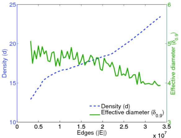
This particular plot was generated for the Wikipedia growth network dataset.  As predicted, the diameter (green curve) is shrinking, while the density (purple curve) is increasing.  Regardless of the actual behavior of each dataset, we would like to generate these plots for all datasets in the KONECT project.  However, there are complications:  (1) If we just write a loop over all networks to generate all plots, this will take way too much time.  Instead we want to only generate those plots that have not yet been generated.  (2) We must restrict the plotting to only those datasets that are temporal, i.e. for datasets that don’t include timestamps, we cannot generate this plot.  The Stu snippet takes care of both aspects.  Let’s now look at the dependency:

@diadens.[dat/NETWORKS_TIME]

As always in Stu, if a name starts with a @, it is a transient.  In this case however, it is a little bit more complex than what we have seen before.  In this case, brackets [ ] are used.  What is the purpose of the brackets in Stu?  They indicate that part of the name is to be generated dynamically.  In this case, it means that Stu must first build  dat/NETWORKS_TIME (which is a file because it does not start with @), and then the brackets [dat/NETWORKS_TIME] will be replaced by the content of the file dat/NETWORKS_TIME.   The file dat/NETWORKS_TIME is a file of KONECT which contains the name of all datasets which have timestamps, all names being separated by whitespace.  This is exactly the list of datasets to which we want to apply our calculation.  In fact, the main.stu file of KONECT also contains a rule for building the file dat/NETWORKS_TIME, which has to be regenerated whenever new datasets are added to the project.  Now, we said that Stu will replace the string [dat/NETWORKS_TIME] with the content of the file dat/NETWORKS_TIME — this is not 100% precise.  Since that file contains multiple names (one for each dataset), Stu will duplicate the whole dependency @diadens.[dat/NETWORKS_TIME], once for each name in the file dat/NETWORKS_TIME.  As a result, the dependencies of @diadens will be of the form @diadens.XXX, where XXX is replaced with each dataset of KONECT that has timestamps.  This exactly what we want:  We have just told Stu that in order to build @diadens (i.e., build all diameter-density plots), Stu must build all @diadens.XXX plots (i.e., each individual diameter-density plot), for each dataset with timestamps individually.  Then, what is the difference between that one line of Stu script, and a loop over all temporal datasets, generating the plots for all datasets in turn?  For one, Stu is able to parallelize all work, i.e., it will be able to generate multiple plots in parallel, and in fact the number of things to execute in parallel is determined by the -j options to Stu (which should be familiar to users of GNU or BSD Make).  Second, Stu will not always rebuild all plots, but only those that need to be rebuilt.  What this means is that when Stu is invoked as

$ stu @diadens

on the command line, Stu will go through all temporal datasets, and will verify whether: (1) the plot has already been done, and (2) if is has already been done, whether the plotting code has changed since.  Only then will Stu regenerate a plot.  Furthermore, because the file dat/NETWORKS_TIME itself has a rule for it in the Stu script, Stu will automatically check whether any new datasets have been added to the KONECT project (not a rare occasion), and will generate all diameter-density plots for those.  (Users of Make will now recognize that this is difficult to achieve in Make — most makefiles would autogenerate code to achieve this.)

Now, let us continue in the script:

@diadens.$network: plot/diadens.a.$network.eps;

Again, this is a rule that spans a single line, and since it ends in a semicolon, doesn’t have a command.  The target of this rule is @diadens.$network, a transient.  What’s more, this target contains a dollar sign $, which indicates a parameter.  In this case, $network is a parameter.  This means that this rule can apply to more than one target.  In fact, this rule will apply to any target of the form @diadens.*, where * can be any string.  By using the $ syntax, we automatically give a name to the parameter.  In this case, the parameter is called $network, and it can be used in any dependency in that rule.  Here, there is just a single dependency:  plot/diadens.a.$network.eps.   Its name does not start with @ and therefore it refers to a file.  The filename however contains the parameter $network, which will be replaced by Stu by whatever string was matched by the target of the rule.  For instance, if we tell Stu to build the target @diadens.enron (to build the diameter-density plot of the Enron email dataset), then the actual dependency will be plot/diadens.a.enron.eps.  This is exactly the filename of the image that will contain the diameter-density plot for the Enron email dataset, and of course diameter-density plots in KONECT are stored in files named plot/diadens.a.XXX.eps, where XXX is the name of the dataset.

Finally, we come to the last part of the Stu script snippet, which contains code to actually generate a plot:

plot/diadens.a.$network.eps: 
        m/diadens.m 
        $[ -t MATLABPATH]
        dat/stepsi.$network 
        dat/statistic_time.full.(diameter avgdegree).$network
{
        ./matlab m/diadens.m 
}

This is a single rule in Stu syntax, which we can now explain line by line.  Let’s start with the target:

plot/diadens.a.$network.eps:

This tells Stu that the rule is for building the file plot/diadens.a.$network.eps.  As we have already seen, the target of a rule may contain a parameter such as $network, in which case Stu will perform pattern-matching and apply the given rule to all files (or transients) which match the pattern.  Let’s continue:

        m/diadens.m

This is our first dependency.  It is a file (because it does not start with @), and it does not contain the parameter $network.  Thus, whatever the value of $network is, building the file plot/diadens.a.$network.eps will always need the file m/diadens.m to be up to date.  This makes sense, of course, because m/diadens.m is the Matlab code that we use to generate the diameter-density plots.  Note that a dependency may (but does not need to) include any parameter used in the target name, but it is an error if a dependency includes a parameter that is not part of the target name.

The next line is $[ -t MATLABPATH], but in defiance of linearity of exposition, we will explain that line last, because it is a little bit more complex.  It is used to configure the Matlab path, and uses the advanced -t flag (which stands for trivial).  The next line is:

        dat/stepsi.$network

This is a file dependency, and, as should be familiar by now, it is parametrized.  In other words, in order to build the file plot/diadens.a.$network.eps, the file dat/stepsi.$network must be built first.  In KONECT, the file dat/stepsi.$network contains the individual “time steps” for any temporal analysis, i.e., it tells KONECT how many time steps we plot for each temporal dataset, and where the individual “time steps” are.  This is because, obviously, we don’t want to recompute measures such as the diameter for all possible time points, but only for about a hundred of them, which is largely enough to create good-looking plots; more detail in the plots would not make them look much different.  Unnecessary to mention then, that the Stu script of KONECT also contains a rule for building the file dat/stepsi.$network.  Then, we continue for one more target of this rule:

        dat/statistic_time.full.(diameter avgdegree).$network

As before, this target includes the parameter $network, which will be replaced by the name of the dataset.  Furthermore, this line contains a Stu operator we have not yet seen:  the parentheses ( ).   The parentheses ( ) in Stu work similarly to the braces [ ], but instead of reading content from a file, they take their content directly from what is written between them.  Thus, this one line is equivalent to the following two lines:

dat/statistic_time.full.diameter.$network
dat/statistic_time.full.avgdegree.$network

Thus, we see that we are simply telling Stu that the script m/diadens.m will also access these two files, which simply contain the actual values of the diameter and density over time for the given network.  (Note that the density is called avgdegree internally in KONECT.)

Finally, our snippet ends with

{
        ./matlab m/diadens.m 
}

This is an expression in braces { } and in Stu, these represent a command.  A command can be specified instead of a semicolon when something has actually to be executed for the rule.  In most cases, rules for files have commands, and rules for transients don’t.   The actual command is not written in Stu, but is a shell script.  Stu will simply invoke /bin/sh to execute it.  In this example, we simply execute the Matlab script m/diadens.m.  Here ./matlab is a wrapper script for executing Matlab scripts, which we use because pure Matlab is not a good citizen when it comes to being called from a shell script.  For instance, Stu relies on the exit status (i.e., the numerical exit code) of programs to detect errors.  Unfortunately, Matlab always returns the exit status zero (indicating success) even when it fails, and hence we use a wrapper script.

One question you should now be asking is:  How does that Matlab script know which plot to generate, let alone which input files (like dat/statistic_time.full.diameter.$network) to read?  The answer is that Stu will pass the value of the parameter $network as … an environment variable called $network.  Thus, the Matlab code simply uses getenv('network'), which is the Matlab code to read the environment variable named $network.  We thus see that most commands in Stu script don’t need to use their parameters:  these are passed transparently by the shell to any called program.

Finally, we can come back to that one line we avoided earlier:

        $[ -t MATLABPATH]

The characters $[ indicate that this is a variable dependency.  This means that Stu will first make sure that the file MATLABPATH is up to date, and then pass the content of that file to the command, as an environment variable of the same name.  Therefore, such a variable dependency is only useful when there is a command.  In this case, the environment variable $MATLABPATH is used by Matlab to determine the path in order to find its libraries.  The file MATLABPATH, which contains that path as used in KONECT, has its own rule in the KONECT Stu script, because its content is non-trivial.  Had we written $[MATLABPATH] as a dependency, that would be the end of the story.  But that would have a huge drawback:  Every time we change the Matlab path, Stu would rebuild everything in KONECT, or at least everything that is built with Matlab, simply because MATLABPATH is declared as a dependency.  Instead, we could have omitted the dependency $[MATLABPATH] altogether, and simply have our script ./matlab read out the file MATLABPATH and set the environment variable $MATLABPATH accordingly.  But that would also not have been good, because then the file MATLABPATH would never have been built to begin with, when we start with a fresh installation of KONECT.  We could also put the code to determine the Matlab path directly into ./matlab to avoid the problem, but that would mean the starting of every Matlab script would be very slow, as it would have to be generate again each time.  We could made ./matlab cache the results (maybe even in the file MATLABPATH), but since ./matlab is called multiple times in parallel, it would have meant that ./matlab would need some form of a locking mechanism to avoid race conditions.  Instead of all that, the -t flag in Stu does exactly what we want here.  -t stands for trivial, and is used in Stu to mark a dependency as a trivial dependency.  This means that the a change in the file MATLABPATH will not result in everything else being rebuilt.  However, if the file MATLABPATH does not exist, or if it exists but needs to be rebuilt and Stu determines that the command using Matlab must be executed for another reason, then (and only then) does Stu rebuild MATLABPATH.  (For those who know the Make build system:  This is one of the features of Stu that are nearly impossible to recreate in Make.)  Note that there are also flags in Stu that can be used in a similar way:  -p declares a dependency as persistent (meaning it will never be rebuilt if already present), and -o as optional (meaning it is only rebuilt, if at all, if the target file is already present).

This concludes our little tour of a little Stu script snippet.  Fore more information about Stu, you may read these previous blog articles:

• Stu – Build Automation for Data Mining Projects
• An Update on the Stu Build System (Stu 2.5)

You can get Stu at Github:

• Stu – Build automation

For reference, the example in this blog article uses features introduced in Stu version 2.5.  Stu is always backward compatible with previous versions, but if you have a pre-2.5 version installed, then of course these new features will not work.

The words written in italics in this article are official Stu nomenclature.

EDIT 2018-01-29:  fixed a typo

Announcing KONECT.cc – New Website and New Features

It’s been a while since I have blogged about KONECT – the Koblenz Network Collection, and much has happened.  We have implemented many new features, which we want to share with all of you.  But the most important news first is that we have a new address:

http://konect.cc/

→ New KONECT Website at KONECT.cc

We finally managed to have a proper domain associated with the project.  The old URLs are still accessible, but they are massively out of date, and may be taken down in the future – we suggest you update your bookmarks and links to the new address.  URLs are mostly the same as with the old site, so for instance the Slashdot Zoo dataset can still be found at http://konect.cc/networks/slashdot-zoo/ – just replace the domain name.  Some other pages have changed however, in particular we now removed the publications page which was massively out of date.  You can now see a list of papers citing us at Google Scholar instead.

The new website is now 100% generated with Stu 2.5.  What this means is that it is now much easier for us to add things to the website.  The list of statistics and the list of plots are now generated completely automatically, and now includes *everything* we compute, and not just a subset chosen for the website.  We also added a list of categories, which shows all 23 (as of now) categories such as social networks, hyperlink networks, etc.  We have quite a few more features that will be added in the next weeks and months – we will be announcing these on the @KONECTproject Twitter feed.

Adding new datasets is now also streamlined, and quite a few datasets have been added recently.  In particular, we added many datasets from Wikipedia, which brings the total dataset count over a thousand, but also skews the whole collection.  The long-term solution to that is of course to add even more datasets, to make it irrelevant.

What it means for you is:  Keep on sending us new datasets (see how to), and keep on sending us feedback to <jerome.kunegis@unamur.be>.

This week, Jérôme Kunegis is at CIKM 2017 in Singapore, and will give a tutorial on data mining large network dataset collections such as KONECT on Friday (Room “Ocean 9”) – don’t miss this out if you’re at CIKM!

 

 

 

An Update on the Stu Build System (Stu 2.5)

If you are reading my blog you are probably aware that I am often advertising the Stu build system.  This is a piece of software that we are using at the University of Namur to run the KONECT project, as well as many other things.

Version 2.5 of Stu has been released a few days ago, and I want to take this opportunity to come back to my previous post about Stu. In that post, I showed a short example of how to use Stu.  Now, with version 2.5 available, that example has become even shorter and easier to write.  Version 2.5 of Stu is the first version of Stu that implements all three core features of Stu. But before I tell you what these three features are, here’s the updated example:

Example

@all: data-clean.[LANGS].txt;

LANGS = { en de fr pt es ja pl nl }

>data-clean.$lang.txt: <data.$lang.txt cleanup 
{
       ./cleanup
}

What does this do?  This is a Stu script to clean up your datasets. I.e., this is the content of a file ‘main.stu’ in your directory. You would then just call ‘stu’ on the command line from within that directory. In practice, this would be part of a larger Stu script in a data mining project that does much more, such as doing actual experiments, plotting, etc.  In this short snippet, we are only cleaning up our datasets. The details don’t matter for this example, but many data mining projects need to clean up their data as a first step, for instance to remove spam entries for an email dataset, etc.

In this example, we have not only one dataset, but multiple datasets, corresponding to multiple languages, as we would in a study of Wikipedia for instance.  Then, we use the program ‘./cleanup’ to cleanup each dataset.

The syntax of a Stu script consists of a set of rules, in which each rule tells Stu how to generate one or more files.  The example consists of three rules.

Let’s start at the bottom:  the last four lines are a rule for the target named ‘data-clean.$lang.txt’.  This is a parametrized rule:  The actual filename can contain any non-empty string in place of ‘$lang’. In this example, $lang will be the language code, i.e. ‘fr’ for French, ‘en’ for English, ‘nl’ for Dutch, etc.

The list of filenames after the colon (‘:’) are the dependencies.  They tell Stu which files need to be present before the target can be built.  In the case of the last rule shown above, there are two dependencies:  the file ‘data.$lang.txt’ (in our example, the non-cleaned up data), and the file ‘cleanup’ (the program we use for cleaning up a file).

The actual command to be performed is then given by the block in the last three lines.  It is executed by the shell and can do anything, like in this example, calling another program.  Since the rule is parametrized (with parameter $lang), it means Stu will execute the command with the environment variable $lang set to the value as matched in the target name. As a result, the ./cleanup program can simply use getenv(‘lang’) or its equivalent in any programming language to access the value of the parameter.

Another feature of Stu we can see here is redirection, written as ‘<‘ and ‘>’.  These are used to redirect the standard input of the command (with ‘<‘) and the standard output of the command (with ‘>’). As a result, our program ./cleanup does not need to access any file directly; it can simply do its filtering from stdin to stdout.

But let’s look at the other two rules in our example.  The rule

LANGS = { en de fr pt es ja pl nl }

is what we call a hardcoded rule.  It simply assigns a predefined content to a file. In this case, we just use that file to store the list of languages in our experiments.

The first rule is a little more interesting now:

@all: data-clean.[LANGS].txt;

It contains brackets (‘[‘ and ‘]’), which I will explain now.  Brackets in Stu mean that a file (in this case ‘LANGS’) should be built, and then its contents inserted as a replacement for the brackets.  In this case, since the file ‘LANGS’ contains multiple names (all the language codes), the filename ‘data-clean.[LANGS].txt’ will be replaced multiple times, each time with ‘[LANGS]’ replaced by a single language code.  As a result, the target ‘@all’ will have as dependencies all files of the form ‘data-clean.$lang.txt’, where $lang is a language code taken from the file ‘LANGS’.

Finally the symbol ‘@’ is used to denote a so-called transient target, i.e. a target that is not a file, but is simply represented as a symbol in Stu.  Since the target @all is not a file, there is no command to build it, and therefore we simply use ‘;’ instead of a command.

Comparison with Make

Readers who know the tool Make will now draw comparisons to it. If Stu was just a rehash of Make, then I would not have written it, so what are the differences?  In short, these are the three core features of Stu:

• Parametrized rules:  Like $lang in the example, any rule can be parametrized.  This can be partially achieved in some implementations of Make (such as GNU Make) by using the ‘%’ symbol. But crucially, this does not allow to use multiple parameters. In the KONECT project, we use up to four parameters in very reasonable use-cases.
• Dynamic dependencies: These are written using brackets (‘[‘ and ‘]’) and have the meaning that the dependency file is first built itself, and then its contents are parsed for more dependencies.
• Concatenation: I haven’t mentioned concatenation yet, but we have used it in the example.  Simply by writing ‘data-clean.[LANGS].txt’, the string ‘data-clean.’ will be prepended to all names in ‘LANGS’, and ‘.txt’ will be appended to them.

These are the three core features of Stu, which set it apart from virtually all other such tools. In fact, I initally wrote Stu in order to have the first two features available. The third feature came to me later, and since I implemented it in Stu 2.5, it now feels second nature to use it.  As a general rule, the three features interact beautifully to give very concise and easy to understand scripts.  This is the raison d’être of Stu.

Comparison with Other Build Tools

There are many build tools in existence, and some of the features of Stu can be found in other such tools.  The combination of the three core features is however unique.  In fact, I have been using Make and Make replacements for years, for KONECT and other projects, always looking for possibilities to express complex dependencies that arise in data mining projects nicely.  Finally, I started writing Stu because no tool was adequate.  In short, almost all Make replacements fail for me because (1) they are specific to a certain programming language, and (2) they are specific to the task of software building.  For data mining projects, this is not adequate.  For those tools that are generic enough, they do not implement the three core features.

By the way, I have been using the Cook tool by the late Peter Miller for years.  Among all Make replacements, it is probably the one that comes closest to Stu.

Stu inherits the tradition of Make replacements having cooking-related names (brew, chef, cook, etc.), and at the same time honors the author and inventor of the original UNIX Make, Stuart Feldman.

Design Considerations

The design considerations of Stu are:

• Genericity: In many projects, the same rule has to be executed over and over again with varying parameters. This is particularly true in data mining / data science / machine learning and related areas, but also applies to simply compiling programs with varying compiler options, etc. Being able to do this using a clean syntax and friendly semantics is the main motivation of Stu, and where virtually all other
  Make replacements fail. Most Make replacement force the user to write loops or similar constructs.
• Generality: Don’t focus on a particular use case such as compilation, but be a generic build tool. There are no built-in rules for compilation or other specific applications. Instead, allow use case-specific rules to be written in the Stu language itself.  Most Make replacement tools instead focus on one specific use-case (almost
  always compilation), making them unsuitable for general use.
• Files are the central datatype. Everything is a file. You can think of Stu as “a declarative programming language in which all variables are files.” For instance, Stu has no variables like Make; instead, files are used. Other Make replacements are even worse than Make in this regard, and allow any variable in whatever programming language they are using. Stu is based on the UNIX principle that any persistent object should have a name in the file system – “everything is a file.”
• Scalability: Assume that projects are so large that you can’t just clean and rebuild everything if there are build inconsistencies.  Files are sacred; never make the user delete files in order to rebuild things.
• Simplicity: Do one thing well. We don’t include features such as file compression that can be achieved by other tools from within shell commands. List of files and dependencies are themselves targets that are built using shell commands, and therefore any external software can be used to define them, without any special support needed from Stu. Too many Make replacements try to “avoid the shell” and include every transformation possible into the tool, effectively amassing dozens of unnecessary dependencies, and creating an ad-hoc language much less well-defined, and let alone portable, than the shell.
• Debuggability: Like programs written in any programming language, Stu scripts will contain errors. Stu makes it easy to detect and correct errors by having much better error messages than Make. This is achieved by (1) having a proper syntax based on tokenization (rather than Make’s text replacement rules), and (2) having “compiler-grade” error messages, showing not only what went wrong, but how Stu got there. Anyone who has ever wondered why a certain Make rule was executed (or not) will know the value of this.
• Portability: Embrace POSIX as an underlying standard. Use the shell as the underlying command interpreter. Don’t try to create a purportedly portable layer on top of it, as POSIX already is a portability layer. Also, don’t try to create a new portable language for executing commands, as /bin/sh already is one. Furthermore, don’t use fancy libraries or hip programming languages. Stu is written in plain C++11 with only standard libraries. Many other Make replacements are based on specific programming languages as their “base standard”, effectively limiting their use to that language, and thus preventing projects to use multiple programming languages. Others even do worse and create their own mini-language, invariably less portable and more buggy than the shell.
• Reliability: Stu has extensive unit test coverage, with more than 1,000 tests. All published versions pass 100% of these tests. All language features and error paths are unit tested.
• Stability: We follow Semantic Versioning in order to provide syntax and semantics that are stable over time.  Stu files written now will still work in the future.
• Familiarity: Stu follows the conventions of Make and of the shell as much as possible, to make it easier to make the switch from Make to Stu. For instance, the options -j and -k work like in Make. Also, Stu source can be edited with syntax highlighting for the shell, as the syntaxes are very similar.

That’s All Good!  How Can I Help?

If you want to use Stu – go ahead.  Stu is available on GitHub under the GPLv3 license.  It can be compiled like any program using the “configure–make–install” trio (see the file ‘INSTALL’).  I am developing Stu on Linux, and am also using it on MacOS.   We’ve even had people compiling it on Windows.  If you try it, I will be happy about hearing from your experiences, and also happy for bug reports.

If you want to see Stu in action, have a look at the Stu script of KONECT.  It controls the computations of all statistics, plots and other experiments in the KONECT project, and runs essentially continuously at the University of Namur.  In practice, I also use Stu for all side projects, generating my CV, writing papers, etc.

In the next months, I will write a blog entry about common anti-patterns in data science, and how they can be avoided using Stu.

More Blog Articles about Stu

• Stu – Build Automation for Data Mining Projects
• The Build System Stu in Practice

Big Table of Binary Fluorine Compounds

While not as common as for instance oxygen, the element fluorine (F) reacts and forms compounds with almost all other elements.  In fact, fluorine is the most electronegative element (except for the unreactive neon on one particular electronegativity scale), and this gives it particular properties:  The pure element, the gas F₂, is extremely reactive, so much that it will react with almost all materials except a few noble gases (such as neon), certain other unreactive substance (such as nitrogen at standard conditions), and compounds that already contain fluorine (such as teflon).  In fact, the history of fluorine is highly interesting in itself, having claimed the death of more than one chemist who tried to isolate the pure element.

The following table gives an overview of the binary compounds of fluorine.  It shows compounds that contains the element fluorine (F) and another element.  The compounds are arranged by oxidation state and stoichiometry, showing that many elements form multiple compounds with fluorine.  Since fluorine is more electronegative than all elements with which it forms binary compounds, all compounds are called “fluorides”, the exception being fluorine azide (FN₃).

Chart as PNG – Chart as PDF

• The table contains links to all Wikipedia articles, or to research papers if the Wikipedia article does not exist yet
• The compounds are coloured according to their type:  molecular compounds in blue, ionic compounds in black, etc.  The exact legend is given within the plot.
• As a bonus, we also include the binary fluorine minerals.

Please post additions and corrections here.

UPDATE:  Version 6

How to Pronounce German Vowels

The German language may be known for its many consonants, but what most learners have trouble with are in fact the vowels.

The following chart gives a pretty much thorough account of the pronunciation of German vowels, in form of a flowchart.  It will help you determine how to pronounce the vowels in a given word.

Chart as PDF

UPDATES

• This is version 5 of the chart, as of 2017-02-17.
• Uploaded version 6, as of 2021-10-27

Please comment here with suggestions, corrections, etc.

A Mathematical Riddle

I’ll just place this here:

You have to compute this expression.

This riddle was composed a few months ago for a competition, but we decided to not use it in the end.  Actually, it is easier than it seems:  You don’t need any calculator or computer to solve it.  A piece of paper (or two) should be enough.  We wrote the riddle in a way that there are several shortcuts that can be used to solve it, but if you don’t find the shortcuts, you can still solve it in the obvious way, taking just a little bit longer.

Also, you have to find the exact answer, not a numerical approximation.

I’m not posting the answer here for now.  If you’re curious whether your answer is correct, post below.

 

No Hairball – The Graph Drawing Experiment

→ QUICKLINK TO THE EXPERIMENT

Many graph drawings look like a hairball.

The larger a network is, the harder it is to visualize it.  Most graph drawing algorithms produce a giant “hairball”, in which nodes and edges are hopelessly mixed up, leaving no way to discern any structure whatsoever. Here is an example:

This is from one of my own papers (WWW 2009), so I should know what I am talking about. Nowadays, I wouldn’t put such a picture in paper, let alone on the first page as I did then.  Many papers however, still contain such graphics.

Can we learn anything from this drawing?  No.  There are no communities visible.  No clustering is apparent.  I cannot even tell whether the graph is bipartite.  In fact, I cannot even estimate the size of the graph from this picture.

So, why do we keep putting hairballs in our papers?  Maybe, because they give us the illusion of insight into a complex network.  Yes, we would like to understand whether a graph displays clustering, bipartivity, assortativity, dissortativity, skewed degree distributions, and a myriad of other interesting properties that complex networks can have. What better way to visualise these features, than by drawing the graph?  Isn’t every visualisation also a drawing?

No, visualisations are not necessarily drawings.  We don’t need to draw a graph in order to visualise it.  In fact, the mere fact that we try to draw the entirety of a network in a small space is what leads to the hairball problem to begin with: Hundred of thousands, millions or even more nodes and edges are crammed into the space of only a few centimetres.  It is no wonder we don’t see anything in a hairball graph:  Each node and each edge gets allocated a space on the order of a micrometre or less – much too small to even be shown on computer displays or printed on paper, let alone seen by the human eye.

What then, can we do to avoid hairballs?  Several ideas have been tried:

• Show only a subset of the network.  This is called sampling.  In its simplest incarnation, choose a random subset of the nodes, to get a subgraph of the real graph of manageable size.  Then, draw that subgraph.
• Aggregate nearby nodes into single nodes.  This is called coalescing, and also produces smaller graphs, which are then drawn with the usual methods.
• Allow the user to zoom in, using interactive software.  This is nice, but doesn’t give any more insight into the overall properties of the network.

These methods are all suited to particular use cases.  But for visualising overall properties of a graph, these methods fail.  What do these methods all have in common?  They assume that to visualise a graph, you have to draw the graph.  The question thus becomes, Can we go further?  Can we visualise a graph without drawing it?  Almost.

In the experiment we are performing, we don’t draw the graph to be visualised.  Instead, we draw another graph – a much smaller one – which is representative of our graph.  In fact, we throw away all nodes and edges of the input.  Only graph statistics such as the assortativity, the bipartivity, and others are kept, and a completely new graph is created, specifically for visualisation.  Most graph/network researchers now think, How can I see individual nodes and edges of the graph?  The answer is that you can’t; that is the point of the method.  We sacrifice local information in graph in order to make global properties more apparent.

The method is in development, and a paper is upcoming, but not public yet.

We are now performing an experiment to find out how to do this graph visualisation optimally:

TAKE PART IN THE EXPERIMENT

This is an interactive experiment that will ask you to look at graphs, and to answer yes/no questions. In fact, you only have to click on graphs to answer.  However:  You must be knowledgeable in graphs and networks to participate.

This will help our research.  If you want to keep in touch with the results of the experiments, write to <pkumar@uni-koblenz.de>.

If you’re interested in graph visualisation, check out the KONECT project; it has lots of graph visualisation methods based on matrix decompositions.

 

Which Elements are Named After Countries?

This week, names of four newly discovered chemical elements have been announced:

• Nihonium (Nh) for element 113
• Moscovium (Mc) for element 115
• Tennessine (Ts) for element 117
• Oganesson (Og) for element 118

These names are up for being revised in six months. Barring some unexpected development, these names will go down in the chemistry books – and more to the point, nuclear physics book – as the names of the elements that complete Period 7 of the periodic table.

Of these four, one name refers to a country (Japan), one to a region (Tennessee), one to a city (Moscow), and one to a person (Yuri Oganessian). All four names were chosen by the discoverers, and honour the discoverers. While the discovering teams have indeed produced a tremendous work and certainly deserve the honour, I find that type of naming quite unfortunate, and even downright selfish.

This has not always been the case. Most elements were not named for selfish reasons. Some elements were named for their properties, such as hydrogen, oxygen, and nitrogen. Some for materials from which they were extracted: beryllium from beryl, aluminium from alum, calcium from calx, sodium from soda, potassium from potash, boron from borax, silicon from silex, and lithium from stones.  Many were named for the colours of their compounds: chlorine is green, bismuth is white, rubidium is red, caesium is blue-grey, gold is yellow, indium is indigo, iodine is violet, rhodium is pink, thallium is green, chromium is colourful, and iridium has the colour of the rainbow. I find these highly poetical. Not to be outdone, some elements were named after astronomical objects: uranium, neptunium, and plutonium for Uranus, Neptune, and Pluto; cerium after Ceres; selenium after the Moon; and tellurium after the Earth.

In more modern times, many radioactive elements were named for their radioactivity: actinium and radium produce rays, astatine is unstable, technetium is artificial. Others were named for various other properties: bromine and osmium smell, argon is inactive, barium is heavy, neon is new, xenon is foreign, phosphorus carries light, krypton and lanthanum are hidden, and dysprosium is hard to get.

Newer elements however, are not named for their properties, but are simply given a name meant to honour the discoverers.  All non-black cells on the follow periodic table are elements whose names can be traced back to a country:

Periodic table of elements by country referred to in the element name.

The last row, Period 7, is almost completely coloured.

I have made some simplifications in the table:  I count Rutherford as British (by his career), and the Rhine as German. Also, the Curies are Polish here.

Let’s look at the country-based names:  Some are quite innocent, like magnesium and manganese, named indirectly after a Greek region called Magnesia. Copper gets its name from the Island of Cyprus, while Beryllium and Strontium get their names indirectly from places in India and Scotland.

In other cases, chemists have tried to honour their country, such as France (gallium and francium), Germany (germanium), and Russia (ruthenium). Note how nicely gallium and germanium are placed side by side. Also note that while europium is named for a deity, the nearby americium was named consciously after the United States.

The Scandinavian countries have the largest share of elements named after them. Famously, a whopping four elements are named after the tiny Swedish village of Ytterby: ytterbium, yttrium, erbium, and terbium. Scandium is named for Scandinavia, thulium for a mythical Scandinavian region.  Holmium and hafnium are named for Stockholm and Copenhagen, respectively. Nobelium and Bohrium and named after a Norvegian and a Danish person, respectively.

Since World War II, newly discovered elements are named simply after people, or after the countries or regions of discovery. In fact, there has been a dispute between American and Soviet physicists about naming priorities. As a result, we don’t have an element named kurchatovium, even if I learned about it in school. With the four new names, that particular dispute should be considered as settled at a score of 7–7, although I’m sure some people on either side of the debate still hope for more.

While names such as einsteinium, fermium, copernicium, and meitnerium  seem fair, given that the persons were already dead and unrelated to the particular discoveries, it seems to me quite preposterous to give names after living people who are involved in the research.  This was the case for seaborgium and the newly named (and not yet finalised) oganesson. Will all respect for these researchers, I doubt that Glenn T. Seaborg and Yuri Oganessian will go down in history in the same way as Copernicus and Mendeleev. Or Einstein and Meitner. Or Curie and Rutherford.

Also, it seems that the responsable discoverers are not trying anymore to follow latin nomenclature:  “nihonium” deserves to be called japonium. That would also give the much more memorable symbol Jp, coinciding with Japan’s country code. If I were responsible for bettering Japan’s standing in the world, I would lobby for “Jp”. On the other hand, Moscovium sounds very appropriate to me, and I like that tennessine and oganesson use the relevant suffixes for halides and noble gases, even if I doubt their corresponding chemistry is going to be characterised anytime soon.

It seems that the last element named after a concept was plutonium. After the last planet to be discovered at the time, and also after a god. The current research teams would do well to come back to naming new elements after actual properties of the material or at least to find metaphors relating to planets and deities, and not just as a vehicle for advertising their labs and principle investigators. Let’s hope that if elements in Group 8 can be synthesized, we will go back to a more classical naming culture.